
How Much Longer Can This Go On?
How can we systematically find the longest increasing subsequence?Introduction
Suppose given a sequence of distinct numbers, and we ask, what is the length of the longest increasing subsequence?For example, I give you
| 2, 5, 1, 4, 7, 6, 3. |
| 2, 5, 7 2, 5, 6 2, 4, 7 2, 4, 6 1, 4, 7 1, 4, 6 |
So if you think only of short sequences, this will seem easy to answer. I'll demonstrate a graphical method that will help you do the necessary mental calculation quickly. But suppose I give you a sequence of 100 numbers
| 41, 93, 31, 73, 98, 29, 12, 54, 24, 0, 52, 78, 87, 55, 25, 81, 76, 91, 51, 7, 39, 92, 65, 40, 45, 5, 1, 20, 84, 99, 27, 32, 13, 8, 2, 61, 19, 9, 74, 60, 66, 79, 47, 86, 30, 3, 85, 42, 89, 43, 70, 17, 6, 63, 28, 11, 34, 75, 22, 64, 59, 16, 48, 15, 90, 80, 69, 67, 35, 72, 50, 14, 33, 53, 10, 38, 94, 18, 58, 46, 49, 88, 68, 21, 62, 44, 97, 82, 37, 83, 95, 4, 56, 57, 77, 23, 96, 26, 36, 71 ? |
Note: The original posted column was mathematically incorrect (near the end of the Heights section). I wish to thank Luigi Rivara for pointing this out. What follows is now correct.
Part I. Increasing subsequences
Reformulation
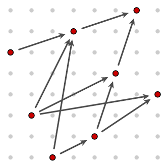
So, suppose we are given a sequence of n distinct integers. It will make things slightly, but not drastically, simpler if we look only at sequences of n integers in the range 0 ... (n-1). In effect we are given a rearrangement or permutation of this range. How can we systematically find the longest increasing subsequence? Let's look at something easier than one of length 100, say this one| 5, | 2, | 0, | 6, | 1, | 4, | 7, | 3 |
| 0 | 1 | 2 | 3 | 4 | 5 | 6 | 7 | |
| 5 | 2 | 0 | 6 | 1 | 4 | 7 | 3 |
We are given a set of such pairs
| [0,5] | [1,2] | [2,0] | [3,6] | [4,1] | [5,4] | [6,7] | [7,3] |
Heights
The diagram also suggests a way to solve the problem systematically.(1) Certain pairs are minimal in the set - there are no smaller pairs. In the diagram, these are the ones that are in some sense 'at lower left'. Here there are three of them: [0,5], [1,2], and [2,0], all marked in red in this diagram:
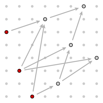
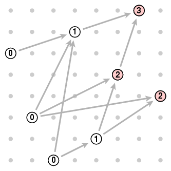
More generally, suppose we call the height of a pair one more than the length of the longest increasing chain ending at it. The minimal pairs are those of height 0. And we have now found a new way to formulate the original problem - we want to find a pair with the largest possible height. Here are the height assignments, which we find by inspection:
The basic principle for any set of pairs is that a pair (x,y) has height h if (a) there is a pair of height h-1 which is less than (x,y) and (b) there are no smaller pairs of height ≥ h. Why is this? Well, a pair of height h-1 has to it a chain of length h, so (a) guarantees that there is a chain to (x,y) of length h+1, and its height is at least h. As for condition (b), if [x,y] were assigned height ≥ h+1 there would be a chain to it of length ≥ h+2, and in that chain just before it a pair of height ≥ h. So there would have to be some pair of height h that is smaller than [x,y].
These criteria are practical. It might seem with condition (b) that we are just going around in circles, but in fact there is a fairly simple way to assign heights as we read from left to right. (1) The very first pair in the list has to have height 0, it is guaranteed to be minimal. (2) Suppose we want to assign height to a pair [i,n] and we have already assigned heights to all previous pairs. Any pair smaller than the current pair [i,n] has to be one of the previous pairs. So we scan them to check conditions (a) and (b).
For example, let's look at our example again. Suppose we have assigned heights for the first five pairs, and want to find the height of the sixth pair [5,4]..
| Index | 0 | 1 | 2 | 3 | 4 | 5 | 6 | 7 | |
| Number | 5 | 2 | 0 | 6 | 1 | 4 | 7 | 3 | |
| Height | 0 | 0 | 0 | 1 | 1 | 2 |
Here are the final height assignments:
| Index | 0 | 1 | 2 | 3 | 4 | 5 | 6 | 7 | |
| Number | 5 | 2 | 0 | 6 | 1 | 4 | 7 | 3 | |
| Height | 0 | 0 | 0 | 1 | 1 | 2 | 3 | 2 |
The obvious drawback of this process is that it is horribly inefficient, since in assigning hi we have to search through all i-1 predecessors. The amount of work involved is thus proportional to 1+ 2 + 3 + ... (n-1) = n(n-1)/2 for a sequence of length n. For n large, this is roughly n2/2; for n=100 about 5,000, not feasible to do by hand.
Organization
Is it really necessary to scan through all nj with j < i when assigning hi ?If you think carefully about what's going on, you see that there are two criteria to be satisfied when assigning height h to ni :
| (1) | ni < all predecessors nj with hj ≥ h ; | |
| (2) | ni > at least one predecessor nj with hj = h-1 ; |
We can understand this better if we maintain a record of all the items with a given height, which I'll do in a kind of bar graph. If the original sequence we are considering is the one above - i.e.
| 5, | 2, | 0, | 6, | 1, | 4, | 7, | 3 |

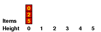
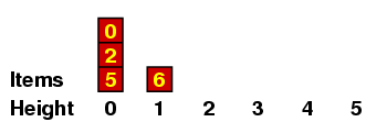
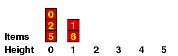
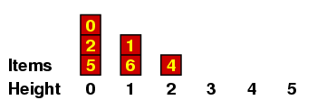
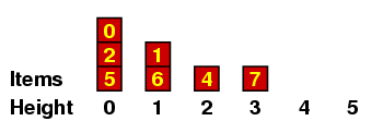
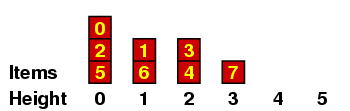
Let me explain a few of these. (a) When we are placing the 2, we have no predecessors of size < 2, so it gets height 0. (b) When we are placing the 6, there are several of size < 6, all of height 0, so it gets height 1. (c) When we are placing the 3, it is < 7 so it can't have height 4 ; and it is < 4, so it can't have height 3 ; but it is > 1, which has height 1, so it gets height 2.
This procedure is much, much better than the original one. It costs a little extra effort to keep the height records, but the amount of time it takes to assign all heights is very roughly proportional to the length of the input sequence.
The sequence of 100 integers written down at the beginning is entirely feasible. We get the length of a longest subsequence to be 15, and a subsequence of that length to be
| 9 | 26 | 34 | 45 | 52 | 55 | 71 | 72 | 75 | 79 | 80 | 92 | 93 | 94 | 95 | |
| 0 | 1 | 2 | 3 | 6 | 11 | 14 | 33 | 38 | 46 | 49 | 56 | 57 | 77 | 96 |
Bumping
The way this computation is usually explained is in terms of the bumping algorithm. We are given a sequence of N distinct numbers ni and want to find the longest increasing subsequence. We start with an empty array h indexed by -1 ... N. We initialize it by setting h-1= -∞ and hi = ∞ for all i ≥ 0.We then progress through the sequence n0, n1, ... modifying the array h as we go along. In terms of the process we described before, at any given moment the j-th item in h will be the previous item we saw of height j. In order to assign a height to [i, ni], we find j with the property hj < ni < hj+1 , and replace hj+1 by ni (i.e. we bump hj+1), to which we assign height j+1. Initializing with -∞ and ∞ saves us some trouble dealing with special cases.
Here's how the array changes with time in the example above.
| h0 | h1 | h2 | h3 | |||
| ∞ | 5,2,0,6,1,4,7,3 | |||||
| 5 | 2,0,6,1,4,7,3 | |||||
| 2 | 0,6,1,4,7,3 | |||||
| 0 | 6,1,4,7,3 | |||||
| 0 | 6 | 1,4,7,3 | ||||
| 0 | 1 | 4,7,3 | ||||
| 0 | 1 | 4 | 7,3 | |||
| 0 | 1 | 4 | 7 | 3 | ||
| 0 | 1 | 3 | 7 |
Part II. Going further
Recycling
The bumping process is rather wasteful. When one inserts an item into the array to replace an item that is already there - when we bump it - we have not paid any attention at all to the item we replace. Is it really necessary just to throw away all those bumped items? Not at all! They can be reused! We build up a new sequence of pairs from the bumped items. If hj < ni < hj+1, we bump hj+1 and replace it by ni. But now instead of just forgetting hj+1, we add the pair [i,hj+1] to a new sequence of pairs to be dealt with in the next stage. In the example above, [1,2] bumps 5; [2,0] bumps 2; [4,1] bumps 6; and [7,3] bumps 4. So the new sequence of pairs we get is [1,5], [2,2], [4,6], [7,4].We insert this into a new blank row. The row becomes 2,4, giving in turn a bumped sequence [2,5], [7,6]. Repeat. If we write the succesive rows underneath each other, we get finally the pattern
| 0 | 1 | 3 | 7 | |
| 2 | 4 | |||
| 5 | 6 |
So far, we haven't done anything with the first coordinates we carry along. Now what we do is maintain at each stage two rows simultaneously, getting eventually two tableaux of the same shape. Whenever a number is added to the first row instead of replacing a number already there, we place the index of the number inserted to the second row. What we get in this example is a similar tableau:
| 0 | 3 | 5 | 6 | |
| 1 | 4 | |||
| 2 | 7 |
Going backwards
The process of going from the initial sequence through a sequence of pairs to a pair of tableaux can be reversed. For example, suppose we are given the tableaux| 0 | 2 | 3 | ||
| 1 | 4 |
| 0 | 1 | 3 | ||
| 2 | 4 |
| 0 | 2 | 4 | ||
| 1 |
| 0 | 1 | 3 | ||
| 2 |
The Robinson-Schensted correspondence
Since we can go both ways - sequence to pair of tableaux and back again - we get in the end a matching of permutations of 0 ... (n-1) with pairs of tableaux of n elements each. This turns out be a remarkable way to understand permutations. This topic has generated a huge amount of mathematics research.To find out more ...
- W. Fulton, Young tableaux, Cambridge University Press.
Chapters 1 - 4 are all about the same topic. I prefer a less abstract approach, but this is easy to read and full of examples.
- C. Greene, Some partitions associated with a partially ordered set, Journal of Combinatorial Theory 29 (1976), 69 - 79.
This is one simple way in which the approach described here can be extended. Greene's algorithm finds maximal increasing chains in arbitrary finite partially ordered sets.
- D. E. Knuth, Permutations, matrices, and generalized Young tableaux, Chapter 31 of Selected papers on discrete mathematics. Original to be found in Pacific Journal of Mathematics 34 (1970), 709-727.
This has many insights not to be found elsewhere in the literature.
- D. E. Knuth, The Art of Computer Programming Volume III, section 5.1.4 on Tableaux and involutions.
This is perhaps the best place to start in learning more about the correspondence between permutations and tableaux.
- C. Schensted, Longest increasing and decreasing subsequences, Canadian Journal of Mathematics 13 (1961), 179-191.
I believe this to be the first place where the problem of longest increasing subsequence was attacked by the methods explained here. But Knuth's paper is clearer.
- J-Y. Shi, The Kazhdan-Lusztig cells in certain affine Weyl groups, Lecture Notes in Mathematics 1179.
The partition of the group of permutations into pieces according to the shape of the corresponding tableau is part of a much larger topic, one in which research is still active. This is perhaps the single best place to start learning about it. Much of Shi's book is concerned with extending Schensted's algorithm to some infinite groups. The ideas introduced in the paper by Greene mentioned above play an important role.
- J. Michael Steele, Variations on the monotone subsequence theme of Erdős and Szekeres, in Discrete Probability and Algorithms, edited by Aldous, Diaconis, and Steele. Published by Springer, 1995.
One of the most interesting questions in this topic is, what is the average length of a maximal increasing subsequence in a sequence of n numbers? The answer is, about 2 √ n. This article discusses this and other related matters.
- Wikipedia entry on longest increasing subsequence.
School Choice
It may come as a surprise that mathematics is increasingly used in situations of this kind to elicit true information....Introduction
Part of good parenting is wanting to maximize the opportunities that are available for one's children. One adage in this spirit is "To get a good job get a good education." So for parents, a good education begins with the schools that a young child attends as he/she is growing up. For those not rich enough to consider private schools and for parents with the freedom to do so, often getting the best possible school for one's child is finding a place to live where the local school - the neighborhood school - is a good one. However, especially in many urban areas many neighborhoods have schools which are poorly regarded by parents, or became so after a family moved to a particular school district. School officials, partly with the view that competitiveness among schools would increase their quality, started to offer parents choice about where they could send their kids. (Although kids sometimes are involved or consulted about where they want to go - more so for high school students than elementary school students - in practice, the politics of school choice involves pleasing parents.) However, if parents are allowed to choose any (public) school in a city or a geographic area they wish, there may be a drastic imbalance between which schools parents would like their children to go to and the number of places that a given school has to accept students.Another complicating factor is that although parents may be aware of the choices for schools available to their children, they may not know how best to use this information. For example, they may not understand the way that information about their preferences among several school choices are actually used. Thus, they may, when asked to give information to a school system about what schools they would like their children to attend, be tempted not to give their true preferences but mis-report their true preferences in the expectation that this misrepresentation will actually help their child get a better school assignment than would otherwise have been the case.
It may come as a surprise that mathematics is increasingly used in situations of this kind to elicit true information. Mechanism design is the area of mathematics and economics that is concerned with issues of this kind. The idea is to design a system which by the nature of its operations encourages people to "disclose" information which is private to them (i.e. give truthful information) because otherwise they will be "hurt." If an organization announces in advance certain information, there are times when one can use mathematics to show that mis-reporting information in such a situation is to one's advantage. However, there are circumstances where using mathematical ideas, typically from the theory of games, one can show that the best response someone has to the way a system is designed is to act in a truthful way. When this truthful way is not only of benefit to the individual but also to a broader community (society), something important has been accomplished.
Two-sided markets
Here we will begin with a general discussion of mechanism design in a relatively narrow class of situations, but situations which nonetheless frequently affect us directly or indirectly. The kinds of situations involved are often referred to as matching problems or two-sided markets. The type of market we have in mind is not the kind of situation where random buyers and sellers interact but a "centralized market" where two kinds of agents are "paired." The basic idea is that one has two groups of "players," though it is not always the case that the players actively compete against each other. Perhaps we have boys and girls at a school dance who have to be paired off, or perhaps a central clearing house to match together students at a college who wish to join a sorority or fraternity. In real-world versions of these market problems one important consideration is that the market clears, that is, players involved get some form of satisfaction by providing matches for all those who desire them. In the school choice setting this means that every student gets assigned to some school, hopefully a highly preferred school, and the schools get as many students as they truly want.The example we will use here is that of school choice. One group of players is the parents of children who need to be placed in schools. The other set of players are the schools the students will enroll in. In practice, the individual schools may not select the students to attend but the decision may be made by a single player, the "school system." Thus, we have a centralized system for doing the pairings.
Before discussing the way mathematics comes into the school choice environment, first let me give some additional highly studied examples of two-sided markets (matching problems). Every year students who graduate from various professional programs such as medical schools need to be matched with hospitals which offer initial employment and additional training for the medical school graduates. These positions are know as residencies. Medical school graduates try to get residencies in cities they find it attractive to live in and at hospitals which are seeking someone with their particular area of interest (family medicine, neurology, psychiatry, etc.) or which are perhaps affiliated with famous universities or medical schools. The hospitals, on the other hand, want students with particular specialties and perhaps better-than-average grades.
There is a long history of "markets" to match medical school graduates and medical residents in both the United States and Great Britain (though in Britain the terminology is not the same as in the US). To fill in more detail of what is involved we have a situation where in essence the hospitals rank the students and the students rank the hospitals. For simplicity here we will assume that the rankings which are produced do not have ties. How does one handle that there may be students whom no hospitals want and hospitals that no students want? Is there a way to deal with the fact that some hospitals might rather have positions unfilled than take some students? Might there be some hospitals that a student would rather not be matched with at all? Yes, this situation can be handled but here we will shortly look at how the matching procedure can be carried out in its simplest form.
Matching problems of this kind come up, with similarities and differences in the situations when:
- boys are to be matched with girls for a school dance
- students are applying to colleges which have preferences for who gets admitted
- students apply to fraternities or sororities with preferences on each side
- students who apply for housing at a university and must be matched to available housing stock
- people who are willing to donate a kidney to someone who needs a transplant and people needing a transplant
- law school graduates who apply for a court internship and judges seeking interns.
Again, before returning to the school choice problem, let me say a bit about the simplest of these models and show how there is a very elegant theory of such markets from a mathematical perspective.
For simplicity let us use the terminology of men and women. Suppose that there are equal numbers of men and women and that we want to pair off men and women, as at a dance. Sometimes the language of "marriage" - proposals and rejected proposals is used here. We will assume each man ranks each of the women without indifference and each woman ranks each of the men without ties.
By way of a specific example, Figure 1 shows 4 men, names m1, ...., m4 who have ranked the four women w1, ..., w4, while Figure 2 shows the rankings that the 4 women ranked by the men, give the men. This particular notation was developed by the British political scientist Duncan Black in the context of ranking candidates in an election. The arrows show the direction of preference, more preferred towards the top. There are many notations for the ways of giving preference, in the form of lists or tables. The notation below is perhaps clearer than many but is not typographically succinct.
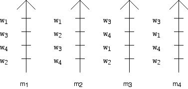
Figure 1
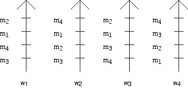
Figure 2
One can give the rankings of the women by the men in a table or matrix form as shown in Figure 3, and the information in Figure 2 is given in matrix form in Figure 4.
| 1st | 2nd | 3rd | 4th | |
| m1 | w1 | w3 | w4 | w2 |
| m2 | w1 | w2 | w3 | w4 |
| m3 | w3 | w4 | w1 | w2 |
| m4 | w3 | w1 | w4 | w2 |
Figure 3
| 1st | 2nd | 3rd | 4th | |
| w1 | m2 | m1 | m4 | m3 |
| w2 | m4 | m1 | m2 | m3 |
| w3 | m2 | m1 | m3 | m4 |
| w4 | m4 | m3 | m2 | m1 |
Figure 4
This notation also takes up a lot of room, so a variety of condensed notations that involve lists ordered from left to right, with preferred "mates" appearing further to the left are used. Such notations make it easier to enter data for large problems into computers so they can be solved quickly. Other notations have been developed that preprocess the information in the preferences so that the algorithms involved in finding "good" matches are speeded up.
One way to match men to women would be to just set up pairs at random. However, if we do this it is not very likely that any particular individual will be happy with whom they were assigned to. However, just to get the flavor of what is going on here, consider the matching:
m1 with w3
m2 with w2
m3 with w1
m4 with w4
Note that this is exactly the same matching as:
w1 with m3
w2 with m2
w3 with m1
w4 with m4
The only thing that has changed is the order in which the man or woman in a pair is listed first.
Consider the pairing (matching) w2 with m2. Note, w2 is m2's second choice and m2 is w2's 3rd choice. Who is m2's first choice? This would be w1 as can be seen by consulting Figure 3. Now, whom is w1 paired with in the current matching? She is paired with m3. By consulting Figure 4 we see that m3 is her 4th choice. So had we paired m2 with w1, these two individuals would be happier than they are with the current pairing. Assuming that the "jilted" people now pair, we have:
m1 with w3
m2 with w1
m3 with w2
m4 with w4
Thus, there is the risk, in some matchings, that two individuals will break their current pairing to get together. When one or both of the individuals in a pairing P, say person p, would rather be paired with someone else, q, than the person they are paired with, and q would rather be paired with p than with q's current "mate," the pairing P is called unstable (with respect to the current matching). Matchings which include unstable pairings seem to be undesirable because it makes "divorce" possible. There is no guarantee that unstable pairs will break up but the potential is there. So if we can avoid such pairs in a matching, this would seem to be highly desirable.
Starting with a random pairing, if all the pairs in this matching are stable we might be happy but we might wonder if there are unstable pairs and if we can break these pairs to get a new matching. In the example above we got rid of an unstable pairing but there is no guarantee that the new matching pairs are all "stable." In fact, it turns out that one cannot be certain that this approach results in a stable matching eventually because one can move from one new matching to another, each time breaking up an unstable pairing but eventually going around in a cycle to a matching one has been at previously.
Is there a procedure (algorithm) which starts with preference tables such as those in Figure 3 and Figure 4 and which can guarantee that when the procedure terminates we have a stable matching? The surprising and amazing answer is "yes!"
The theory of stable marriages and how to find them basically goes back to Lloyd Shapley and David Gale. The question was originally posed by Gale, and Shapley provided an algorithm.

(Photo of David Gale courtesy of the University of California at Berkeley News Center)

(Photo of Lloyd Shapley obtained from Wikipedia)
David Gale did important work in mathematical programming, mathematical economics, and game theory. Lloyd Shapley is one of America's most prominent game theorists. The game solution concept known as the Shapley Value is named for him.
Literally hundreds of theoretical and applied research papers have grown out of the work of Gale and Shapley. These papers are shaped by people with expertise in mathematics, computer science, economics, business, and many other areas of expertise. Two significant contributors to different aspects of the Gale-Shapley circle of ideas are Robert W. Irving and Alvin Roth. They have contributed by collaborations with many people and working with many students and colleagues (see references for their many joint and solo publications).
(Photo courtesy of Rob Irving)
(Photo courtesy of Al Roth)
Their work has ranged over a wide range of variants, pure and applied, of Gale-Shapley models. Roth comes at these questions from the perspective of an economist and Irving from that of a computer scientist. More and more we are getting insight into pure and applied aspects of the Gale-Shapley model via a broader and broader range of skills and interests on the parts of the people who investigate these problems.
Vanilla Gale-Shapley
Here is how the algorithm (a step-by-step procedure, guaranteed to terminate in a finite number of steps) that Gale and Shapley developed works. It is sometimes called the Gale-Shapely Marriage Algorithm or, as we will sometimes refer to it here, the deferred acceptance algorithm. The basic idea is that either the men "propose" to the woman (or vice versa). At a given stage of the algorithm, say where the men propose, a woman will have no men to choose from or several. If there are several, a woman chooses the best of these but there is a possibility that from her perspective someone better may come along later, so if she has a choice she only accepts her best suitor provisionally (we are assuming there are no ties). Only at the end will the algorithm guarantee that every man will be matched with some woman, and that all the matches will be stable!Rather than describe the algorithm in abstract general terms we will work through a specific example (the one coded in Figures 3 and 4 above), from which it should be clear how the algorithm works in general. We will consider first how the Gale-Shapley algorithm works when the men "propose" to the women. Later, we will consider the version where the women "propose" to the men. The algorithm will progress in "rounds." At the start, each woman is sitting behind a desk (say in a gym). In each round each man will "propose" to some woman. A particular woman may get no suitors or several. If she gets none, she waits until a future round when a suitor will appear. (There are variants of this algorithm where men might rather be single than paired with any particular woman, and women might prefer to be single than paired with any particular man, in which case one has to modify what is described here.) Each round begins with a signal (say, a bell). When the bell rings any man who has not been provisionally accepted by some woman goes to the highest woman on his list who has not already rejected him. Women who get proposals pick provisionally the highest man on their list from the suitors who show up.
For our example, with the men proposing, here is what happens:
Round 1:
m1 proposes to w1 as does m2, while both m3 and m4 propose to w3.
Now, w1 has two suitors m1 and m2. Since she prefers m2 she provisionally accepts him (and her other suitor m1 will have to try the next woman on his list in the next round). Similarly, w3 accepts m3 (since she prefers m3 to m4) and m4 will go on to a lower preference choice in the next round.
Round 2:
m1 will propose to w3 and m4 will propose to w1.
Now w3 was provisionally matched with m3 so she now has to pick between him and her newly arriving suitor m1. Since she prefers m1 to m3, she lets go of m3 and provisionally accepts m1.
Also, w1 was provisionally matched with m2 and now m4 also arrives as a suitor. Since m2 is, in fact, her first choice, she sends m4 on to a lower choice.
Round 3:
Both m3 and m4 propose to w4. Previously, she had no suitors. She prefers m4 and so m3 will try to find acceptance from some lower choice. The other two women (w1 and w3) will continue to the next round with their provisional choices.
Round 4:
Now, m3 tries w1 (who provisionally has m2) and given her current choices she again stays with m2 and m3 must again try for a lower choice.
Round 5:
m3 tries w2. Since she has no suitors she accepts him, and we now have a matching since no woman has several suitors.
This matching is:
w1 with m2
w2 with m3
w3 with m1
w4 with m4
Is this match stable? The theorem that Gale and Shapely proved indicates that it must be. Furthermore among all matchings that can be found which are stable, each individual male is as well off as he can be in any stable matching and each woman is as badly off as she can be in any stable matching! When the men propose we get a "male optimal" and "woman pessimal" matching, already a perhaps surprising consequence of doing the mathematics.
What happens when the women propose? Following the same procedure as above but with the men behind the desks and the women moving around as required, we get the matching:
m1 with w1
m2 with w2
m3 with w3
m4 with w4
By symmetry, it is perhaps not surprising that this stable matching is favorable to the women at the "expense" of the men. This matching is woman optimal and male pessimal.
It is not difficult to extend this basic theory to the case where some men would rather not be paired with any of the available women and some women would rather not be paired with the available men. Furthermore, for the case where the men are "students" and the women are "hospitals" and we seek to fill hospital positions with students, we can allow for the hospitals to have more than a single slot to be paired with, so we can think of the hospitals as having quotas or positions to be filled.
In conjunction with the matching situation for hospitals and medical students, a bit generalized for allowing students or hospitals to be matched with themselves (which from a student point of view there are hospitals which they will turn down by preferring to be matched with "themselves" rather than go to these hospitals), we can get an insight into the way that the desire for stability interacts with society's goal of having hospitals in rural and/or unpopular cities get desired staff.
Theorem: If students and hospitals have strict preferences in ranking each other, the set of students who get offers and the set of hospitals which get their positions filled are the same for every stable marriage!!
This means that stability has very important implications for students who have characteristics that might be "unpopular" and "hospitals" that have characteristics which might be unpopular. We can't remedy the situation by moving to some other stable pairing. Furthermore, there is also this remarkable theorem (due to A. Roth) which sheds light on using the Gale-Shapley "theory" in applied settings:
If students and hospitals have strict preferences, and if a particular hospital does not get all of the students it wishes (i.e. fill the quota of seats that it wants to have filled) in some specific stable matching M, then for all other stable matchings it will have exactly the same set of students!
These theorems have the effect that those hospitals which have trouble finding doctors to come to them cannot solve their situation by "tinkering" with the way a stable matching is picked out from the set of stable matchings. There is a trade-off between having stability and getting these hospitals to have their quotas filled when there is a broad perception they wold not be a good place to work.
Stable matchings
The Gale-Shapley algorithm can be run with either the boys proposing or the girls proposing, and in either case a stable matching exists, and in some rare cases it is also the same matching. However, in general, as in the example above, the two matchings one gets are different. Because of the elegance of the Gale-Shapley ideas and procedures and the strong symmetry of what happens for this algorithm, it may be tempting to think there are not a lot of stable marriages possible for "general" preferences of the men and women. However, this is definitely NOT the case. Although there are lots of lovely results about the number of stable marriages when there are n people involved, there are still lots of open questions.Let's begin with the example of the preference tables below. How many stable marriages do you think there are in this case? (This example is due to Dan Gusfield and R. Irving.) It turns out there are 10 stable marriages.
| 1st | 2nd | 3rd | 4th | |
| m1 | w1 | w2 | w3 | w4 |
| m2 | w2 | w1 | w4 | w3 |
| m3 | w3 | w4 | w1 | w2 |
| m4 | w4 | w3 | w2 | w1 |
| 1st | 2nd | 3rd | 4th | |
| w1 | m4 | m3 | m2 | m1 |
| w2 | m3 | m4 | m1 | m2 |
| w3 | m2 | m1 | m4 | m3 |
| w4 | m1 | m2 | m3 | m4 |
Stable marriages:
1234 (male optimal), 2134, 1243, 2143, 2413, 3142, 3412, 4312, 3421, and 4321 (woman optimal)
John Conway (as reported by Donald Knuth) called attention to the fact that the collection of all stable marriages forms an algebraic structure called a "distributive lattice." Intuitively, this systematically offers a way to "order" the stable marriages which lie "between" the male optimal and female optimal stable marriages. Furthermore, though it is still an open problem to count the largest number of stable marriages in terms of the number of people in the market n, it is known that for every n which is a power of 2, there are preference tables for the men and women where there are at least 2n-1 stable marriages. (For example, for n = 8 (eight men and women rank each other), this theorem says there is an example with 128 stable marriages.)
It would be nice to know for a given n the formula for the largest number of stable marriages. Furthermore, one might not care too much if there are lots of stable marriages for some "weird" set of preferences. What might really matter is what happens for either "typical" cases or "random" cases. Not surprisingly scholars have taken an interest in questions of this kind not only because they seem interesting from a theoretical point of view but because there are also practical concerns about how much "freedom" there is to find a stable marriage. When might finding a stable marriage be like looking for a needle in a haystack? (In the simplest version of Gale-Shapley problems we know there are typically two (at least 1) stable matchings, the male and female optimal ones. However, in some extensions of the basic model there is no guarantee that stable marriages exist. Yet, in practice, for large markets (ones with lots of players) there often seem to be stable marriages even though the theory does not guarantee this.
Borrowing from issues that have turned out to be important in other areas involving fairness questions (elections and fair division) we might ask what the consequences are of the men and women "mis-reporting" their true preferences. For example, if one has information about other men's likes and dislikes, a particular man might believe that if he misrepresents his true preferences he might be better off. Roth has shown that under fairly general assumptions about the nature of a two-sided market there is no "stable" matching mechanism design where stating one's true preferences always makes each player (hospital or student) better off. On the other hand, when one of the parties to a matching situation (say the school system) is not an active but a passive player, then one can under some circumstances design a mechanism which encourages the student side of the market to be truthful.
The most studied interaction between ideas related to the Gale-Shapely model and settings in which two-sided markets actually exist has been in the area of placing doctors seeking "residencies" with hospitals, or the equivalent situation in Great Britain. A variety of systems using different algorithms have actually been set up and implemented. The fascinating discovery has been that when these matching systems obeyed the requirement of stability, they "worked" while when the did not obey stability they tended to "unravel." What this means is either the hospitals would make commitments earlier and earlier in the education process of the doctors who would years later be seeking hospital placements, or the time that a doctor had to accept a placement would get shorter and shorter to prevent the doctors from negotiating with other hospitals to find what they hoped would be a better placement than the one offered to them. Many fascinating studies have appeared to get insight into why systems that do not guarantee stability might not "unravel" and what is special about those "markets" where, despite the fact that stability is not guaranteed, sometimes the "markets" do not fall apart. This information sets the stage for an interplay between having the theory of two-sided markets be in closer accord with what is planned in advance (versions of deferred acceptance systems in new settings) as well as historically implemented or evolving 2-sided markets.
Another aspect of these placement markets is that the theory has shed light on why it is difficult for rural communities to get doctors to accept placements in their hospitals as mentioned above.
The NRMP (National Residents Matching Program, - which evolved from the NIMP program, National Intern Matching Program) is a voluntary system for pairing doctors seeking residencies and hospitals seeking doctors. NRMP has a long and fascinating history. In response to a market which was "chaotic," this matching system was developed; it used an algorithm which led to stable matchings though the approach was not that of the Gale-Shapley work which came later. For a long time the system used the hospital optimal approach but the system has evolved to its current algorithm in a variety of ways to deal with being more "student" friendly and also to deal with the problem of "couples." Theory shows that when one tries to expand the Gale-Shapley model to deal with couples, one can produce examples where stability is not always guaranteed. Nonetheless steps can be taken to avoid having the market break down in a way that handles couples much of the time. NRMP has approved new changes in the way its system works (to start in 2011).
School choice
In the school choice environment there has been a fascinating and developing interplay between "theory" and "applications." Whereas the original deferred acceptance algorithm was formulated within the context of having n men and n women rank each other with strict preferences and no truncation (there was no possibility of being unmatched), the school choice environment does not allow the "vanilla" version of Gale-Shapley to be implemented. It was originally formulated so that no woman (or man) would rather be "not married" than paired with the particular choice of men (women) she (he) faced, and thus, had to make some choice among the persons available. Over the years there have been many extensions and generalizations of the theory that is associated with the basic Gale-Shapley model that we have described here. In particular, one realistic extension to the school choice case allows schools to rank groups of students equally and students to be indifferent between several schools.To give some of the flavor of what happens in a realistic version of the school choice problem, here is a simplified description of the evolution of what happened in New York City at the high school level. Students typically (together with their parents) must decide at the end of the 8th grade (or for some schools at the end of 9th grade) in which high school to continue their education. Students have the choice of attending a public school, but some will choose to attend a private high school if their family can afford it when they are unable to get an acceptable public high school assignment from their point of view. In the fall of each new academic year, parents and children work to apply for a high school placement for the following year. New York City maintains a system of "neighborhood high schools" but it also has specialized schools which require that students who wish to attend these schools take a special examination. Approximately 90,000 students are involved each year in wanting placements; the specialized high schools have 4000-5000 places. In designing a system to match schools and applicants, the city reached out to experts in the field. There were a variety of considerations that the "mechanism designers" needed to take into account.
These included:
a. Producing stablematchings of students to schools. (The difficulty of having a market using unstable matchings is alluded to above.)
b. Producing matchings which are "efficient" (Pareto optimality kinds of conditions). The issue here is that while a matching might be stable, there would be other stable marriages that some students prefer while other students are no less happy with these other matchings. One can look at "efficiency" from the point of view of all players, only the schools, or only the students. In the background here is that when a relatively simple version of Gale-Shapley that we discussed is used in the student propose version, then the students can do no better than with any other stable matching.
c. Having students (parents) report preferences for the schools being applied to honestly, rather than using some strategic reporting of preferences in the hope of getting better placements. Having a system that encouraged honesty would be valuable. (Data from the use of a school choice system in Boston which had been based on a mechanism design different from the Gale-Shapley deferred acceptance approach suggested a discrepancy between the pride being taken by the school system in giving students high ranking choices, and the reality of the satisfaction with actual placement. Thus, the school system claimed high level of satisfaction because the satisfaction was being based on rankings which, in fact, were not true rankings. When polls were taken which compared actual assignments with true rather than "strategic" preferences, the results were much less positive. Eventually Boston changed the system it used to try to avoid problems which had arisen from the system it was using.)
Another issue with respect to the honesty of the expressed preferences which are produced by the participants in the two-sided market has emerged from the analysis of what was done with choice mechanisms in the past. For example, in the school choice environment a school can announce publicly that it has 150 seats, when in fact it really has 200 seats and it plans to use those "hidden" seats in some way outside the matching mechanism to help it fill seats. Researchers are now trying to study how to avoid this situation and get more "transparency."
d. Dealing the assignment of students to specialized schools which have limited capacity.
e. Dealing with ties (although in some cases the schools have preferences for particular students, there are also large groups of students about whom the schools are "indifferent"). The reality is that depending on how ties are broken the students may not be equally satisfied with the outcomes of the different ways ties are broken. Thus, the system by which ties are broken might affect the efficiency of the system in a subtle way. One can break ties using a number assigned to each student at each of the schools or one can assign student tie-breaking numbers for the individual schools differently.
f. Limits to how many schools a student can apply for.
Many school systems have so many choices that it is not realistic to have all the students rank all of the programs. Hence, it seems that it may give better outcomes to limit how many choices the students can make in the number of schools they apply to.
Mathematics evolves because it generates intrinsically interesting internally generated questions and responds to the need to solve problems that arise in fields like business, economics, biology or physics. Jeff Dinitz posed a "pure mathematical" question in 1979 about latin squares which Fred Galvin answered in 1994. The method of solution used the Gale-Shapley model! Unexpected connections of this kind are one of mathematics' great charms. Gale-Shapley's beautiful model continues to grow and be used in response to problems arising in such areas as school choice. These are exciting times for both pure and applied mathematics.
From Pascal's Triangle to the Bell-shaped Curve
In this column we will explore this interpretation of the binomial coefficients, and how they are related to the normal distribution represented by the ubiquitous "bell-shaped curve."...Introduction
Blaise Pascal (1623-1662) did not invent his triangle. It was at least 500 years old when he wrote it down, in 1654 or just after, in his Traité du triangle arithmétique. Its entries C(n, k) appear in the expansion of (a + b)n when like powers are grouped together giving C(n, 0)an + C(n, 1)an-1b + C(n, 2)an-2b2 + ... + C(n, n)bn; hence binomial coefficients. The triangle now bears his name mainly because he was the first to systematically investigate its properties. For example, I believe that he discovered the formula for calculating C(n, k) directly from n and k, without working recursively through the table. Pascal also pioneered the use of the binomial coefficients in the analysis of games of chance, giving the start to modern probability theory. In this column we will explore this interpretation of the coefficients, and how they are related to the normal distribution represented by the ubiquitous "bell-shaped curve."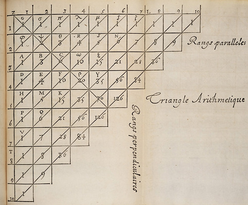
Pascal's triangle from his Traité. In his format the entries in the first column are ones, and each other entry is the sum of the one directly above it, and the one directly on its left. In our notation, the binomial coefficients C(6, k) appear along the diagonal Vζ. Image from Wikipedia Commons.